fw.render_svg

Use fw.render_svg when the result needs a compact figure for a document or a webpage. Choose the visual form that fits the question: a grain map, a census tree, a pair mapping, or a two-way heatmap.

SVG is vector output. It can scale without rerunning analysis, but it can only depict evidence that the analysis actually saved.

Jump to the worked example or the argument reference.

Function reference

fw.render_svg(
    result,
    *,
    section=None,
    detail='full',
    view=None,
    show_exceptions=False,
    max_findings=12,
    shading=None,
)

This page describes Fieldwork 0.3.2. Import the package with import fieldwork as fw. View the documented source.

Arguments

Argument	Type / default	Effect
result	Result or mapping; required	A fw.Result or its to_dict() export. Rendering uses saved evidence and never reruns analysis or accesses the original dataframe.
section	str or None; None	Select a section of a composed result. Overview sections are missingness, dependencies, paths and value_patterns. Profile sections are levels, census, grain and pairs; a profile defaults to grain.
detail	“full” or “topology”; 'full'	"full" includes quantitative evidence. "topology" suppresses quantitative support and selectors in the presentation, while keeping structural labels. It is not anonymization: labels can still identify people or records.
view	str or None; None	Choose a view compatible with the result kind; None uses its default. See the view table below. Other kinds support only None or "findings".
show_exceptions	bool; False	List the columns each key fails to determine in the grain map. It does not retrieve additional source rows and has no effect on other views.
max_findings	nonnegative int; 12	Maximum items per list in the findings view; default 12. Full dependency figures add up to five candidate summaries and this many completed tests, including below-threshold tests. Zero omits these lists. Other views draw the saved evidence within its analytical bounds.
shading	mapping or None; None	Shading ranges for association and joint-count cells, typed as fieldwork.typing.Shading: {"association": rule, "counts": rule} with rule "equal", "log", "quantile" or three increasing cut-offs. None uses "equal" for association and "log" for counts. See shading ranges.

Returns and output choices

Returns an SVG string. Save with Path("figure.svg").write_text(svg, encoding="utf-8"), or display using IPython.display.SVG. The function does not write the file itself. A profile defaults to its grain section; specify a computed section when grain was not requested.

Full dependency presentations include candidate summaries and every completed per-target test within display limits, including tests below the finding threshold. They distinguish observed target coverage from consistency on evaluated rows and repeat-only consistency. Missing-category tests are labeled. Candidate and test lists have separate display bounds; SVG shows at most five candidate summaries. The overview summary stays compact; render its dependencies section for detail. These numerical qualifications are absent from topology.

The grain matrix uses feature rows and candidate-key columns, so adding features extends it vertically. For wide evidence and interactive filtering, use the HTML matrix. SVG wraps full labels and reports each rendered list’s display omissions separately.

Shading ranges

The pairs association view and the joint-count heatmap shade each cell by one of four ranges, and every cell also prints its value. By default the cut-offs adapt to each figure, and the legend prints the ones used.

Rule	Cut-offs	Default for
"equal"	Four equal-width ranges between the smallest and largest value	association
"log"	Four ranges evenly spaced on a log scale up to the largest value (from 1 for counts), rounded	counts
"quantile"	About a quarter of the cells in each range	—
three numbers	Fixed, increasing cut-offs, the same in every report	—

fw.render_svg(counts, shading={"counts": (10, 50, 150)})

Fixed cut-offs keep several reports on one scale. Across the contexts of a pairs result the cut-offs are computed once, so every context uses the same ranges. A value equal to a cut-off falls in the higher range. The same shading argument applies to render_html and visualization_data.

Colour and type

Figures draw on white with dark outlines and use the system’s sans-serif and monospace fonts, with column and key names in monospace. Colour encodes an analysis result and nothing else:

Colour	Meaning
Blue	Determined: constant cells, and n:1 pairs (the row determines the column)
Orange	Varies: varying cells, and 1:n pairs (the column determines the row)
Dark fill, white text	1:1 pairs, determined both ways
Dashed outline	Absent or out of scope: undefined, untested, n:m, missing share, unplaced columns, omitted branches
Yellow → green → teal → petrol	Amounts in four ranges (association, joint counts); teal alone for share bars

Legends sit at fixed places below grids and after bars.

Interpretation and boundaries

An invalid view, section, or detail raises ValueError. Association view requires detail="full". A requested section that was not computed cannot be rendered. An invalid shading rule raises ValueError, and a shading value that is not a mapping raises TypeError.

Available views

Result kind	Default	Alternative	How to read it
grain	map	matrix	Observed determinant structure, or exact candidate/target evidence.
levels	bars	—	Independent level counts and omitted mass.
census	tree	—	Ordered prefix groups; shares use the recorded population.
pairs	mapping	association	Cardinality mapping, or Cramér’s V magnitude.
joint_counts	heatmap	—	Counts in locally supported row/column domains.
Other kinds	findings	—	Availability bars where applicable and bounded evidence cards; schema proposals draw one card per column.

Walkthrough: a seed-library handoff figure

Two library branches have prepared twelve seed packets for a community exchange. A coordinator needs a picture of which seeds each branch will bring, with quantities for packing and a simpler version for discussing the assortment. Each row below is one packet, so row counts also count packets; they do not count varieties or visitors.

Download the runnable example. It follows the same steps and saves the figures in your working directory.

Build a small, auditable inventory

from pathlib import Path

import pandas as pd
import fieldwork as fw

packets = pd.DataFrame(
    [("East", "Beans")] * 4
    + [("East", "Herbs")] * 2
    + [("West", "Beans")]
    + [("West", "Herbs")] * 3
    + [("West", "Flowers")] * 2,
    columns=["branch", "seed"],
)
counts = (
    packets.groupby(["branch", "seed"])
    .size()
    .reset_index(name="packets")
)
print(counts.to_string(index=False))

branch    seed  packets
  East   Beans        4
  East   Herbs        2
  West   Beans        1
  West Flowers        2
  West   Herbs        3

Both branches bring six packets. Across branches, beans and herbs each account for five packets, but their distribution differs. A branch-first census preserves that distinction.

Choose the section before choosing the view

result = fw.profile(packets, ["branch", "seed"], pairs=False)
full_svg = fw.render_svg(result, section="census", view="tree")
Path("render_svg.svg").write_text(full_svg, encoding="utf-8")

fw.profile computes levels and a census for the chosen dimensions; pairs=False skips the pair section. section="census" selects the branch-to-seed analysis; view="tree" chooses its supported drawing. Select the census explicitly here because a profile’s figures default to grain, which we have not requested. A levels bar chart would summarize each column separately and lose the branch-to-seed nesting that matters here.

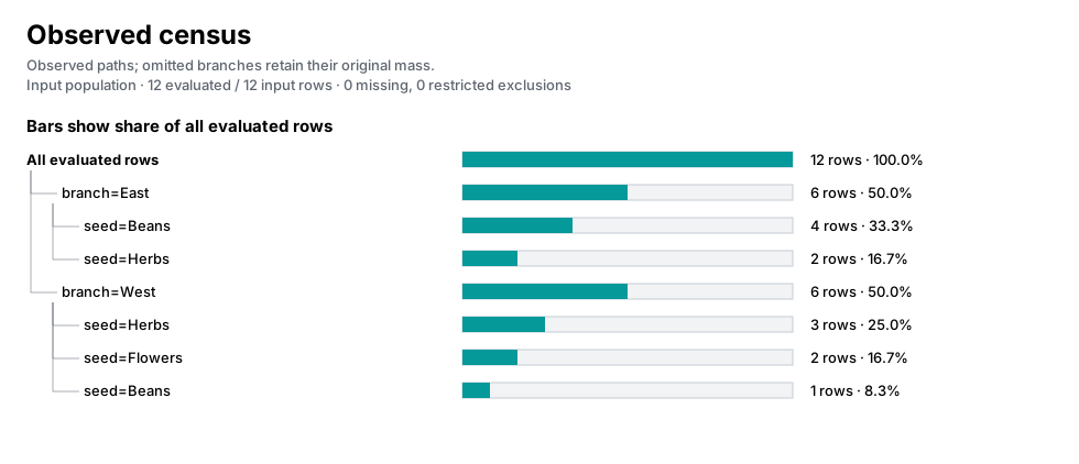
Open render_svg.svg in a browser or insert it into a document. The figure was returned as an SVG string and saved by write_text. render_svg does not save a file or rerun the analysis. The tree includes five observed branch–seed combinations; flowers appear under West only in this inventory.

Read the denominator behind the bars

The full figure’s bars and percentages use the total evaluated population: twelve packets. East’s bean bar therefore shows 33.3%, even though beans make up two thirds of East’s contribution. Inspect the visualization data to report both shares accurately.

figure_data = fw.visualization_data(
    result, section="census", detail="full"
)
leaves = [row for row in figure_data["rows"] if row["depth"] == 2]
for row in leaves:
    print(
        f"{row['parent_label']} / {row['label']}: {row['count']} packets; "
        f"{row['share']:.1%} of all; {row['parent_share']:.1%} of branch"
    )

branch=East / seed=Beans: 4 packets; 33.3% of all; 66.7% of branch
branch=East / seed=Herbs: 2 packets; 16.7% of all; 33.3% of branch
branch=West / seed=Herbs: 3 packets; 25.0% of all; 50.0% of branch
branch=West / seed=Flowers: 2 packets; 16.7% of all; 33.3% of branch
branch=West / seed=Beans: 1 packets; 8.3% of all; 16.7% of branch

These counts describe the prepared packets. They do not establish visitor demand, branch capacity, or why one branch prepared more beans.

Use topology for an assortment discussion

For a conversation about which combinations exist, remove quantitative annotations while keeping the observed paths.

topology_svg = fw.render_svg(
    result, section="census", view="tree", detail="topology"
)
Path("render_svg-topology.svg").write_text(
    topology_svg, encoding="utf-8"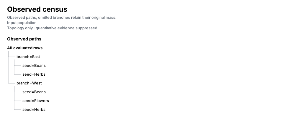
)

Topology answers “which branch brings which seeds?” It cannot answer “how many boxes should we pack?” The source result still contains all twelve packets’ evidence. This is a presentation choice, and labels such as branch and seed names remain visible. Use the full version when quantities drive the decision.

Keep analysis limits separate from drawing choices

A rendering option cannot restore a deeper analysis that was never computed. For example, stopping the census after the branch level produces a six-versus-six summary, without seed children.

shallow = fw.profile(
    packets, ["branch", "seed"], pairs=False, census={"max_depth": 1}
)
shallow_svg = fw.render_svg(shallow, section="census", view="tree")
Path("branches-only.svg").write_text(shallow_svg, encoding="utf-8")

The population stays twelve; the branch-level figure cannot establish which seed combinations occur. Use the original two-level result for the assortment question. Its observed paths also do not define a catalog of permitted combinations: West’s flowers do not prove East cannot prepare flowers.

Choose a figure for the next conversation

Use render_svg.svg when quantities matter and render_svg-topology.svg when discussing the assortment. Keep the original result if you will need a different view later.

Continue exploring

fw.render_html, fw.visualization_data, fw.render_plaintext. See results and configuration for serialization and result-method contracts.